Back to Don's Maps
The Causes of the end of the last Ice Age
The last great ice age began around 120 000 years ago. One massive ice sheet, more than 3 kilometres thick in places, grew in fits and starts until it covered almost all of Canada and stretched down as far as Manhattan. Another spread across most of Siberia, northern Europe and Britain, stopping just short of what is now London. Elsewhere many smaller ice sheets and glaciers grew, vast areas turned into tundra and deserts expanded as the planet became drier.
With so much ice on land, sea level was 120 metres lower than it is today. Britain and Ireland were part of mainland Europe. Florida was twice the size it is now, with Tampa stranded far from the coast. Australia, Tasmania and New Guinea were all part of a single land mass called Sahul. The planet was barely recognisable.
Then, 20 000 years ago, a great thaw began. Over the following 10 000 years, the average global temperature rose by 3.5° C and most of the ice melted. Rising seas swallowed up low-lying areas such as the English Channel and North Sea, forcing our ancestors to abandon many settlements. So what drove this dramatic transformation of the planet?
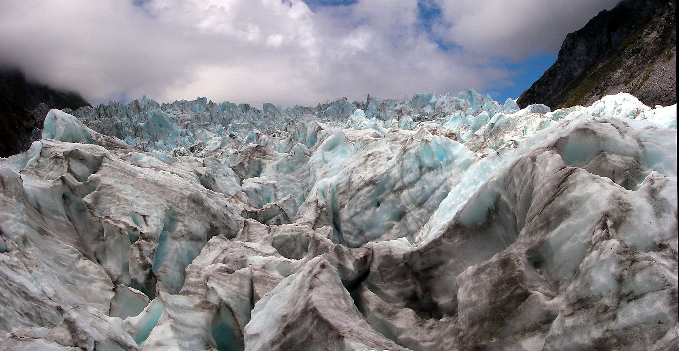
This panoramic photograph of two photos stitched together was taken in the middle of the Fox glacier in New Zealand, in an area of seracs, huge lumps of ice pushed up by pressure as a glacier enters a hollow, or exposed when the glacier passes over a hump in its bed. Glaciers are powerful agents of erosion, as can be seen by the dirt in the ice here.
Photo: Don Hitchcock 2007
We have long known the thaw began with an increase in summer sunlight in the northern hemisphere, melting ice and snow. It is what happened next that has remained mysterious. Soon after the thaw began, for instance, the southern hemisphere began to warm while the northern hemisphere cooled - the opposite of what was expected from the changes in sunshine. Now, after nearly two centuries of wrestling with seemingly contradictory findings, we think we finally understand how the ice age ended.
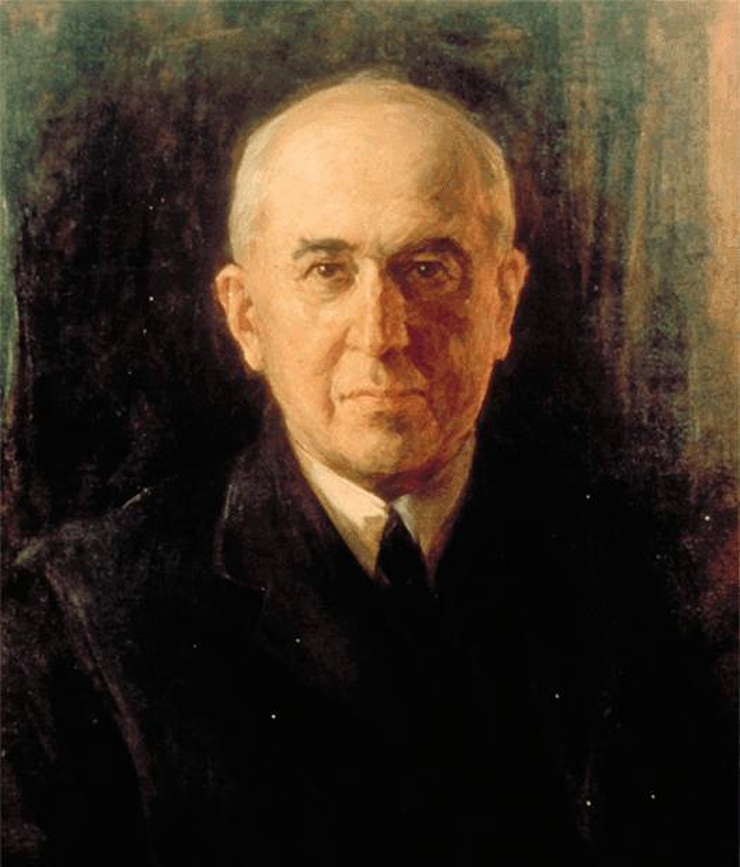
Early in the 20th century, the Serbian astronomer Milutin Milankovitch concluded that summer sunlight in the northern hemisphere must be the crucial factor and spent years painstakingly calculating how this had changed over the past 600 000 years. His ideas weren't accepted at the time, but in the 1970s studies of ocean-sediment cores revealed that the advances and retreats of the ice ages did indeed coincide with 'Milankovitch cycles'.
Photo: http://www.detectingdesign.com/milankovitch.html
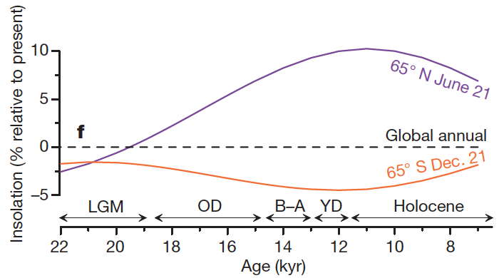
Insolation forcing for latitudes 65°N (purple) and 65°S (orange) at the local summer solstice, and global mean annual insolation (dashed black).
(Here we can see that the forcing of climate warming by the sun (i.e. the Milankovitch cycles) was only for the northern hemisphere.
Other effects were behind the global warming which 'ended' the last ice age, though technically we are still in it - Don )
Photo and text: Shakun et al. (2012)
Yet many enigmas remained. For starters, the changes in sunshine were tiny. Even if they were amplified by more of the sun's heat being absorbed by the planet as snow and ice melted, it was hard to account for the scale of the global changes.
What's more, when summer sunshine increases in the northern hemisphere, it decreases in the southern hemisphere. This had led Croll to suggest that ice ages alternate between hemispheres: when the north freezes the south thaws and vice versa. But it had long been clear that the whole world had warmed at around the same time.
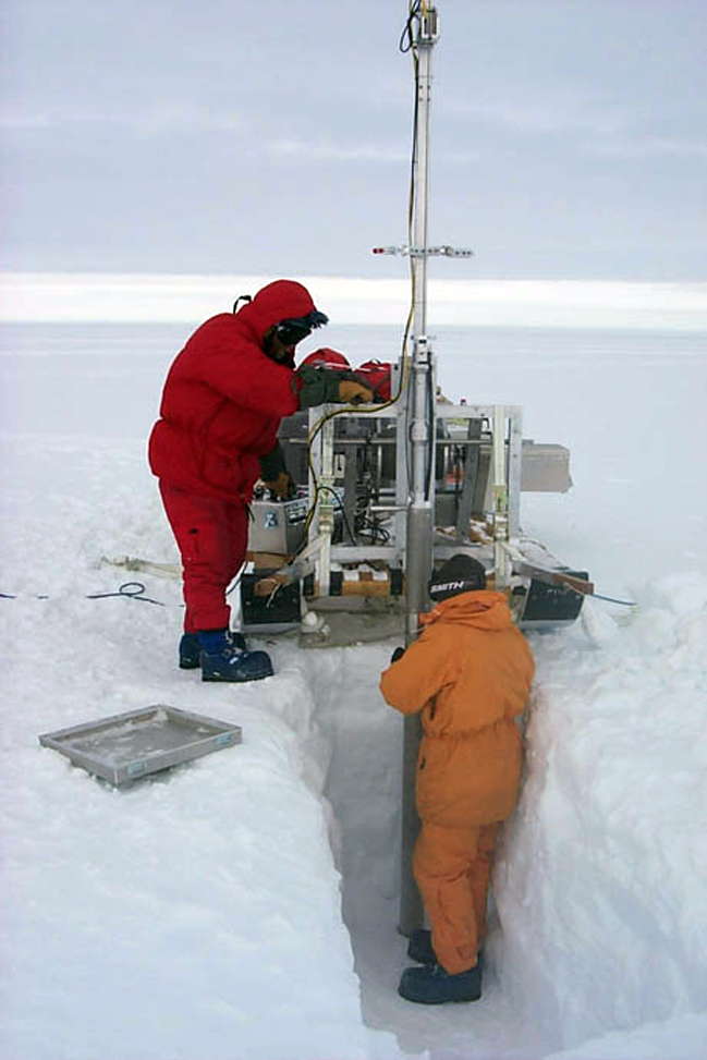
The answer to these puzzles seemed to emerge in the 1980s, when ice cores drilled in Antarctica revealed an astonishingly close correlation between atmospheric carbon dioxide levels and temperature.
'For the last million years, you see these two going up and down, up and down, together through each ice age, and it's almost in perfect lockstep,' says Jeremy Shakun of Harvard University. 'It's about as beautiful a correlation as you ever get from nature.'
Photo: Paul Mayewski drilling in Antarctica, http://www.ediblegeography.com/glacial-terroir/
If CO2 levels had risen soon after the thaw began in the north, it would explain why the southern hemisphere began to warm too. It would also help to explain the magnitude of the changes. But this promising idea ran into a major problem: by around a decade ago, it had become clear that the Antarctic starting warming a few hundred years before CO2 levels began to rise. So while soaring CO2 levels undoubtedly warmed the planet - they are now thought to be responsible for about half of the warming as the ice age ended - they weren't the initial cause. 'Something else was causing Antarctica to warm,' says Daniel Sigman of Princeton University.
Pollen puzzle
This wasn't the only mystery. In the 1930s, studies of sediments containing the pollen of the alpine flower Dryas octopetala and other plants suggested that almost as soon as Europe began warming, it suddenly got cold again. This cold phase, called the Oldest Dryas or Mystery Interval, lasted from around 17 500 years ago to 14 700 years ago. Ice cores later showed Greenland cooled at the same time.
Yet during this period Antarctica warmed steadily. "On the detailed scale, the south seems to warm before the north," says Sigman. But what would make the southern hemisphere warm even as the northern hemisphere cooled? It could not be due to orbital changes or rising CO2 levels - but it could be due to changing ocean currents.
As the vast ice sheets began to melt 19 000 years ago, stupendous quantities of fresh water poured into the North Atlantic (see diagram). Studies of marine sediments off the Irish Sea coast, for example, show that the sea level there rose about 10 metres in just a few hundred years (Science, vol 304, p 1141).
Today in the North Atlantic, salty water arriving from the tropics cools, becomes very dense and sinks to the bottom. These deep, cold waters flow all the way to the southern hemisphere, while on the surface warm water - including the Gulf Stream - flows north. This system of currents is called the Atlantic meridional overturning circulation.
The huge quantities of fresh water pouring into the ocean 19 000 years ago would have diluted the salty water, making it less dense. Result: a slowdown in the overturning circulation. The proof came in 2004 from a study of ocean sediments. The ratio of two heavy elements, which indicates the speed of the deep current, showed that the overturning circulation had almost ground to a halt 17 500 years ago (Nature, vol 428, p 834).
The result was a kind of see-saw effect. With much less heat being carried north by the surface currents, the northern hemisphere cooled. The tropical and subtropical regions of the southern hemisphere, by contrast, began warming as they were losing less heat to the north. This explains many puzzling findings. The slowdown of the Atlantic current can also help explain why CO2 levels rose during the great thaw (see diagram).
By the 1990s, the search for the source of the CO2 was focusing on the Southern Ocean. Isotopes in ocean sediments suggested that a huge reservoir of CO2 had built up in deep waters during the ice age. It is thought that a lack of vertical mixing, along with a cover of sea ice, trapped the gas. During the thaw, however, the ocean was 'uncorked' and much of the CO2 escaped into the atmosphere.
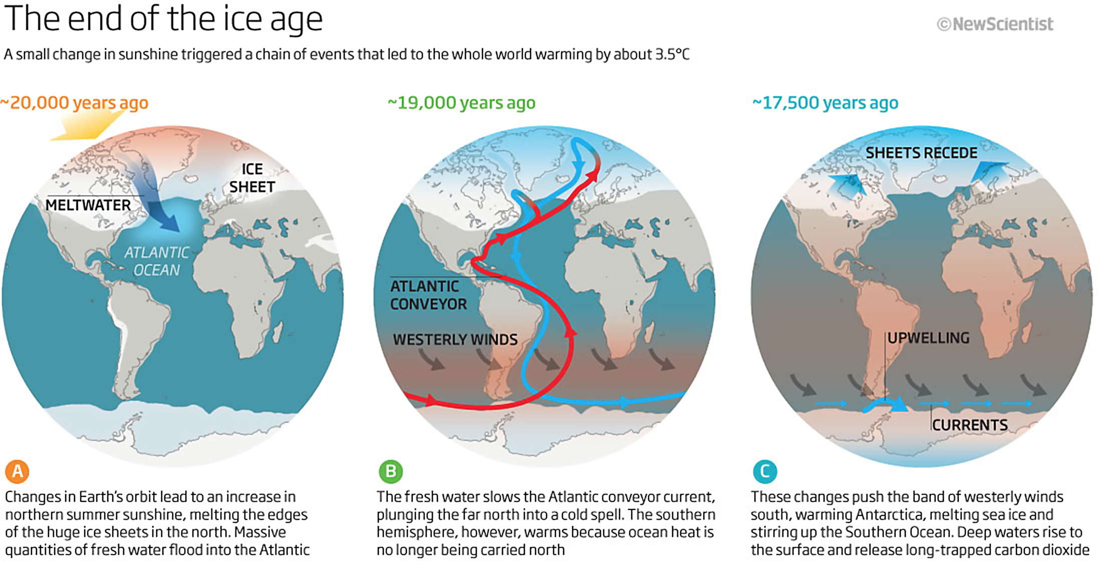
Photo: © New Scientist, http://www.newscientist.com/articleimages/mg21628891.900/1-the-great-thaw-charting-the-end-of-the-ice-age.html
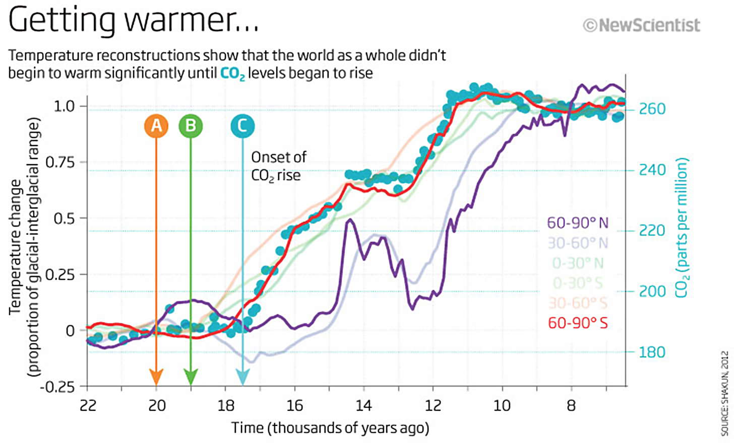
This graph shows what was happening to the temperatures, and is especially useful for interpreting A, B, and C from the illustration above.
At A, changes in the Earth's orbit lead to an increase in northern summer sunshine, melting the edges of the huge ice sheets in the north. Massive quantities of fresh water flood into the northern Atlantic. Meanwhile, the Southern Hemisphere (red line) remains cold.
At B, the fresh water slows the Atlantic conveyer current, which brings warm water to the north. This plunges the far north (purple line) into a cold spell, since this warm water is no longer acting with the increase in summer sunshine to warm the edges of the ice sheets in the north. However, the southern hemisphere warms because with the slow down of the northwards current, it is no longer losing heat, even though there is no increase in summer sunshine, as is happening in the northern hemisphere.
At C, these changes push the band of westerly winds south, accelerating the warming of Antarctica, melting sea ice and stirring up the Southern Ocean, the deepest layers of which had vast quantities of CO2 dissolved in them. When these CO2 rich waters rise to the surface, they release this long trapped CO2, which then starts the process of warming the whole earth. The blue dots show the concentration of CO2 in the atmosphere.
(What I find interesting is that the course of warming in the southern hemisphere shows a relatively steady increase, strictly in line with the rise in CO2 levels, while the temperatures in the Northern Hemisphere (from 30° N to the North Pole) show much more variability, presumably as the result of changes in ocean currents - Don )
Photo: © New Scientist, http://www.newscientist.com/articleimages/mg21628891.900/2-the-great-thaw-charting-the-end-of-the-ice-age.html
Text: adapted from http://www.newscientist.com/article/mg21628891.900-the-great-thaw-charting-the-end-of-the-ice-age.html?full=true
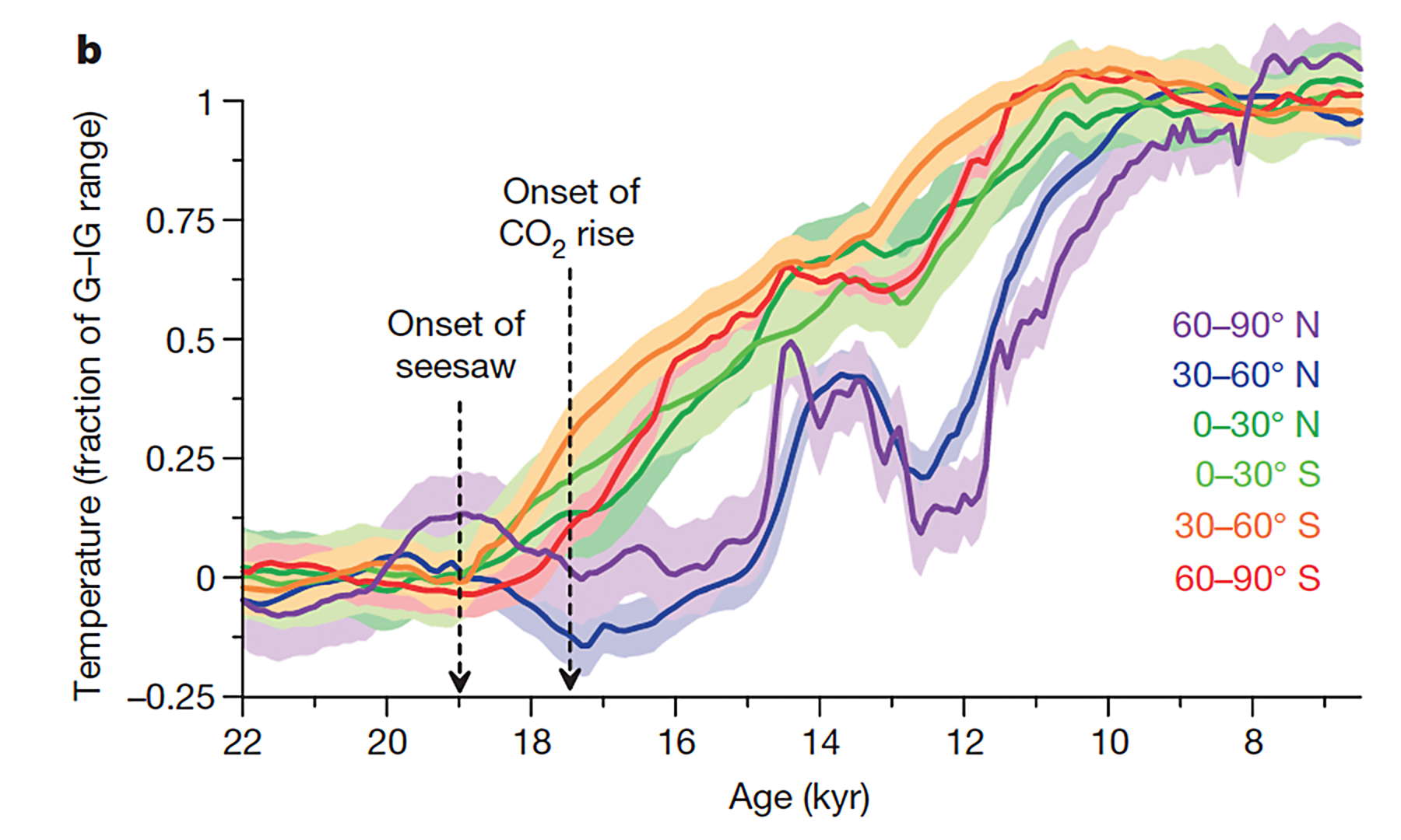
This graph from the authors of the original study shows the graphs more clearly than the one from New Scientist above.
Photo: Shakun et al. (2012)
Around 12 900 years ago, the see-saw swung again. Temperatures in northern latitudes suddenly plummeted and remained cold for about 1 300 years. This cold snap, called the Younger Dryas, is thought to have been caused by a colossal meltwater lake in North America, which held more water than all the Great Lakes put together, suddenly flooding into the Atlantic and shutting down the overturning circulation once again.
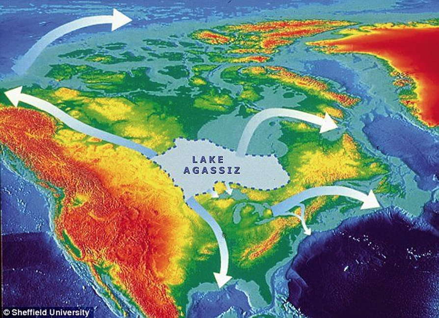
This image from Sheffield University shows the size of Lake Agassiz, though not the ice sheet from which it had formed as meltwater, and which dammed it to the north.
When it got large enough, it suddenly emptied, starting the cold snap known as the Younger Dryas in the Northern Hemisphere when it temporarily shut down the ocean circulation which was until that point helping to end the ice age.
Photo: © Sheffield University
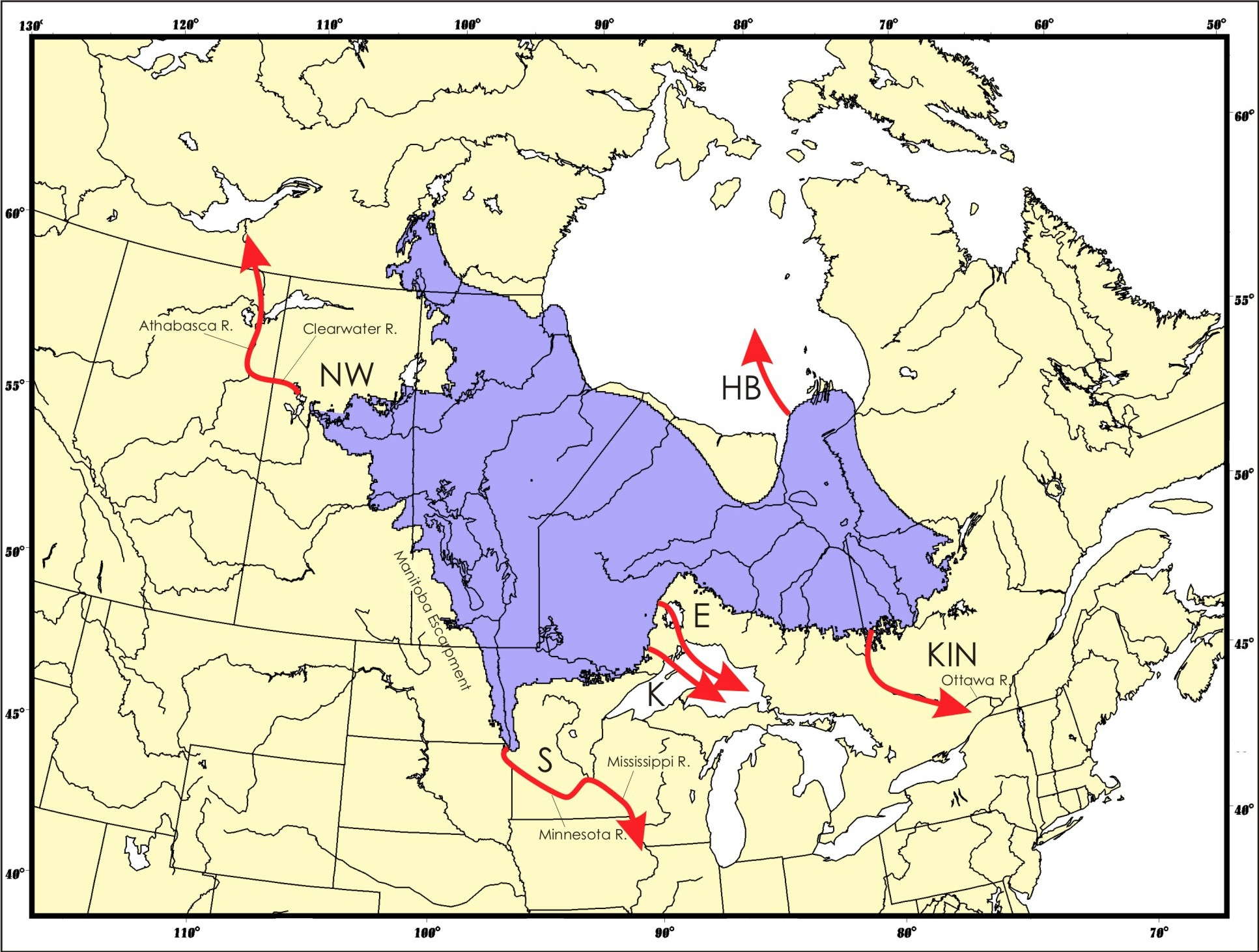
Another map showing the extent of Lake Agassiz.
Approximate total area occupied by Lake Agassiz over its 5000 calendar-year history (purple) (after Leverington and Teller, 2003).
At no single time did the lake occupy this entire area; rather, the waters of the lake gradually shifted northward, following the wasting southern margin of the LIS and possibly combining with Lake Ojibway to the east.
Locations of lake overflow were a function of topography and the position of the confining ice sheet. Major drainage routes: S, Southern outlet to the Gulf of Mexico; K, Kaministikwia route to the Superior basin; NW, Northwestern outlet to the Arctic Ocean; E, Eastern outlet system to the Superior basin; KIN, Angliers and Kinojévis outlets to the St. Lawrence River valley; HB: final release of Lake Agassiz waters into the Tyrrell Sea.
Photo and text: http://www.webpages.ttu.edu/dleverin/quaternary_envs/quaternary_environments.html#agassiz
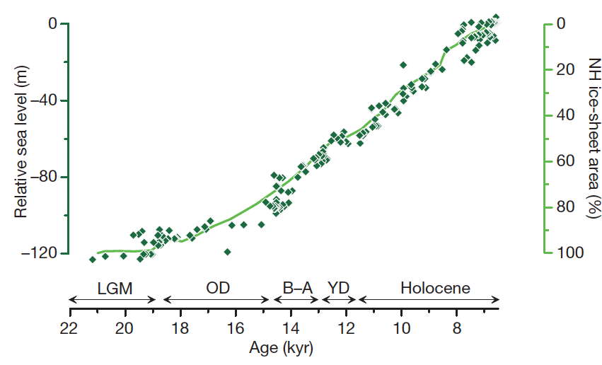
Increase in relative sea level shown in diamonds.
Decline in Northern Hemisphere ice-sheet area shown on the green line derived from summing the extents of the Laurentide, Cordilleran, and Scandinavian ice sheets through time.
(As you would expect, the decline in the size of the ice sheet and the increase in relative sea level are in lock-step - Don )
Photo and text: Shakun et al. (2012)
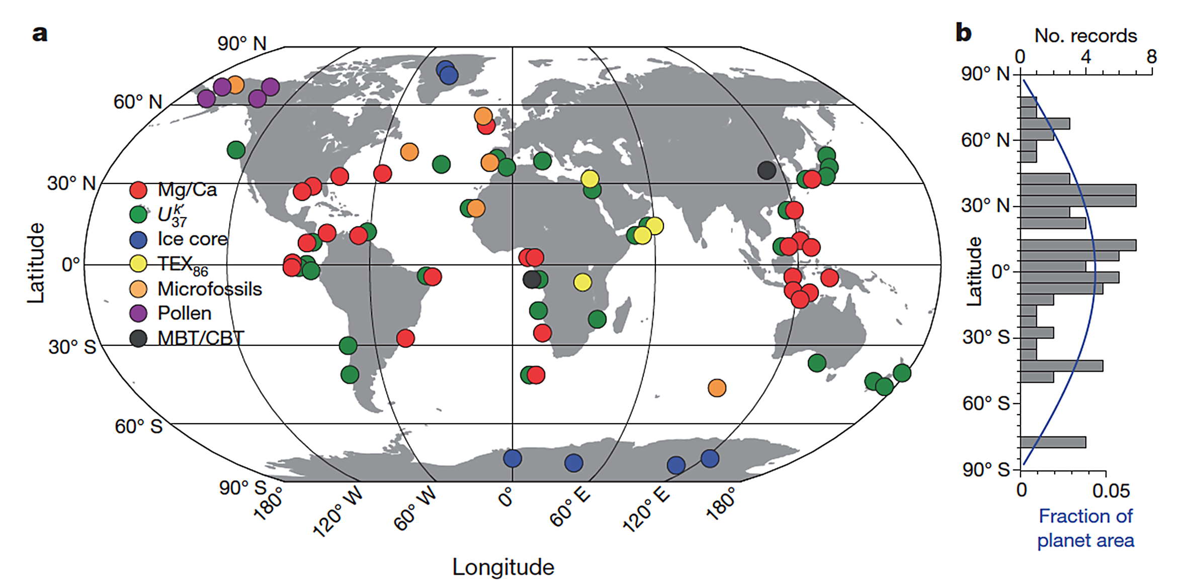
This important map shows where the temperatures for the various latitude groups were obtained.
Proxy temperature records
a, Location map. CBT, cyclization ratio of branched tetraethers; MBT, methylation index of branched tetraethers; TEX86, tetraether index of tetraethers consisting of 86 carbon atoms; Uk'37, alkenone unsaturation index.
b, Distribution of the records by latitude (grey histogram) and areal fraction of the planet in 5° steps (blue line).
Photo: Shakun et al. (2012)
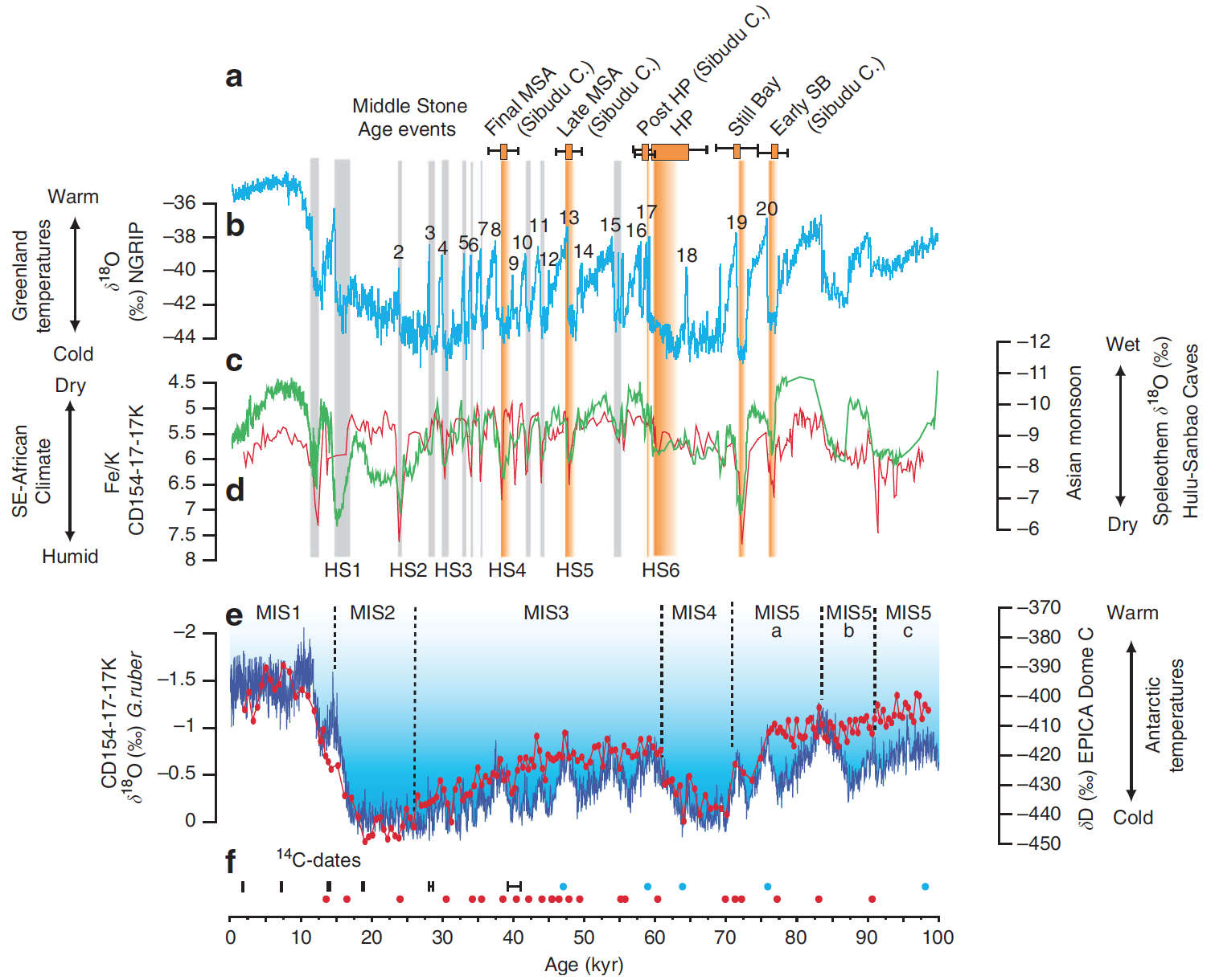
Climate change during the Middle Stone Age in Southeast Africa.
(a) Ages of Southeast African Middle Stone Age events. Error bars indicate 2-sigma ranges, (that is, a 95% confidence level - Don ), coinciding with Heinrich events 4–6 and cold Greenland stadials 19 and 20.
(b) δ18O record from Greenland ice core NGRIP (light blue, Speleo-age model presented in
Barker et al. (2011) displaying abrupt temperature variability in the North Atlantic. Numbers indicate warmer stadials. Underlying bars indicate cold stadials with more extreme Heinrich stadials (HS1–HS6) highlighted
(c) δ18O splice from Chinese speleothems (green) (Hulu and Sanbao Cave)20,48 showing synchronous variability of the East Asian summer monsoon with climate variability in the North Atlantic
(d) Fe/K of CD154-17-17K (red) indicating higher river discharge and wetter Eastern Cape Province climate during Northern Hemisphere stadials.
(e) Planktonic foraminiferal (G. ruber) δ18O record from CD154-17-17K (red), reflecting global ice volume variability and local sea-surface conditions, in comparison with EPICA Dome C deuterium record (blue)35. Marine isotope stages (MIS) are indicated.
(f) Age control points for CD154-17-17K, including radiocarbon dates (black), tuning of the foraminiferal δ18O record.
Photo and text: Ziegler et al. (2013)
References
- Barker, S. et al., 2011, 800 000 Years of abrupt climate variability, Science, 334, 347–351 (2011).
- Leverington, D., Teller, J., 2003, Paleotopographic reconstructions of the eastern outlets of glacial Lake Agassiz, Canadian Journal of Earth Sciences, 40, 1259-1278.
- Shakun, J. et al., 2012, Global warming preceded by increasing carbon dioxide concentrations during the last deglaciation, Nature, 484, 49–54 (05 April 2012)
- Ziegler, M. et al., 2013, Development of Middle Stone Age innovation linked to rapid climate change, Nat. Commun., 4:1905 doi: 10.1038/ncomms2897 (2013).